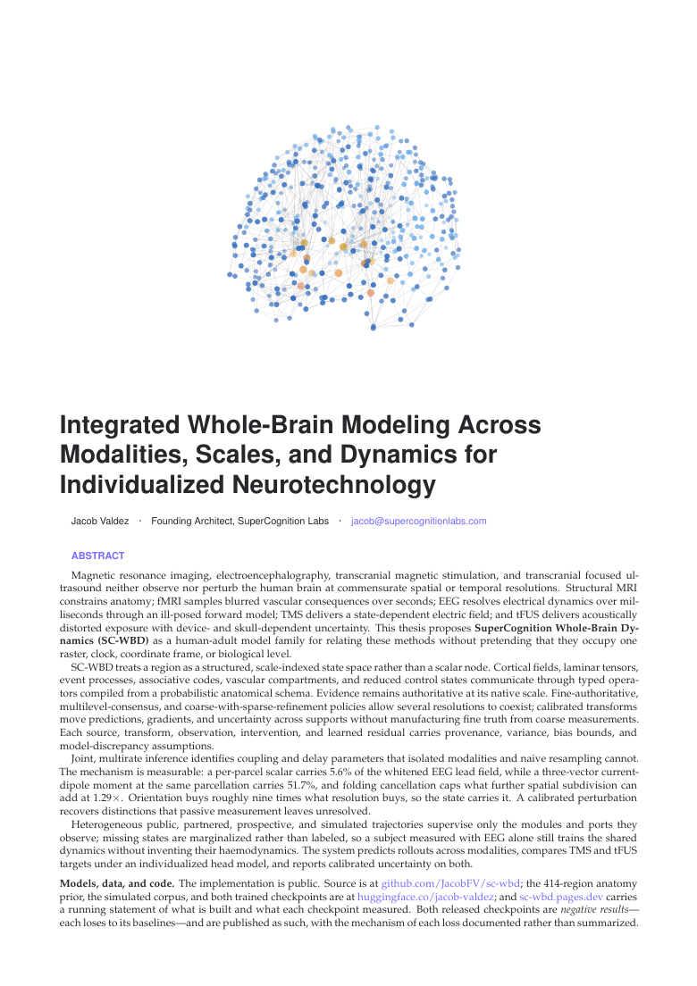
SC-WBD: an integrated whole-brain foundation model across modalities, scales and dynamics
SC-WBD is a working model of one person's brain — 414 regions wired the way theirs are, carrying what is known about each one's chemistry, myelination and timescale. Electrical activity every millisecond, blood flow every two seconds, a magnetic pulse pushing on the tissue, and what the person actually does: each reads the same shared state, through its own physics, on its own clock.
The World's First Whole Brain Dynamics (WBD) Model
Every way of looking at a brain sees something different. Electrodes read it a thousand times a second but can barely say where the signal came from. An MRI scanner sees the whole brain but reads it once every two seconds, and reads blood flow rather than activity. A magnetic pulse or a beam of focused ultrasound goes the other way, pushing on the tissue instead of watching it — ultrasound reaching structures deep enough that no non-invasive instrument can otherwise touch them. Additionally, what a person looks at, or types, or says is not a brain measurement at all, and yet even that information can inform our understanding of a given brain.
Most people are only ever measured one way, so results from each instrument never quite add up, and almost none of them are about any particular brain. SC-WBD keeps one shared model and lets each kind of signal constrain the part it can actually speak to.
Each way of reading the brain gets its own forward model, because each one
measures a different physical quantity. Electrical recording is a
lead field computed from a boundary-element head model, which
carries regional current to each scalp electrode. fMRI is the
Balloon–Windkessel haemodynamic differential equation,
integrated forward so blood-flow signal is predicted from neural state
rather than assumed proportional to it. fNIRS is a photon-path model through
scalp, skull and cortex. What the person does is read at the boundary of the
body and needs no head model at all.1In the package these are
EEGObservationOperator, BOLDObservationOperator,
FNIRSObservationOperator and
BehaviorObservationOperator. Each implements the same interface —
a prediction plus a bias-and-variance ledger — on its own spatial support and
its own clock, and each returns what it does not know rather than a point
estimate that hides it.
They also run on different clocks, and are not resampled onto a common one. The electrical head reads the latent trajectory every millisecond; the haemodynamic head reads the same trajectory once a second or two, through an equation whose own time constants are seconds long. Nothing is interpolated into fictitious equivalence between them — the shared state is what they have in common, and the operators are where they differ. That is what the word integrated is doing in this project's name, and it is also where run 4's fMRI result went wrong: the equation integrates now, and the likelihood it produces still degrades over training.scwbd/observe/__init__.py
None of that starts from nothing. Before any signal arrives the model is conditioned on a measured prior over the same 414 regions: 12,274 tracts between them — 1,618 taken as hard structure, 7,386 soft, 3,270 proposed — at a mean length of 38.8 mm, and 33 maps per region, among them a 19-tracer PET panel of receptor and transporter densities, T1w/T2w myelin, cortical thickness, MEG intrinsic timescale, the principal functional gradients, the sensorimotor–association axis, and cerebral blood flow and glucose metabolism. Every region the model has an opinion about therefore arrives already carrying what is known about its chemistry, its myelination, its timescale and its wiring, and the posterior is conditioned on all of it rather than on the recordings alone.reports/anatomy_prior.md The prior is also published on its own, and each map carries its own licence and citation.
Sorting signals this way is what makes partial data usable.2In the
schema these are stimulus, observation,
boundary_output and context, and the distinction is
enforced: an observation must declare the forward operator it is
measured through, or it is refused. Without that axis, eye tracking and button
presses could only be declared as measurements of neural state, which is a
different and wrong claim. Someone's gaze is real evidence, but it is not a
reading of their cortex, and a model that confuses the two learns the wrong
thing.
400 on the surface + 14 deep inside
plus 33 measured maps per region
weights, data and code all public
against closed-form solutions, to 1.3% or better
New: bWIN EEG 001 and a matched comparison
A task-specific WIN model forecasts 64 future EEG samples from 24 observed samples. On 25 held-out people it improves over zero, while fitted linear and community neural alternatives have lower average error. Both SC-WBD-003 and SC-WBD-004 perform better on the five people held out by both checkpoints. This is a measured comparison of separate research artifacts, not a claim that the new model supersedes the integrated predecessors.
Read the results, actual-data figure, and comparisons with released models · Checkpoint and source
Modelling brain activity
The first thing the model does is the ordinary thing: given what a brain has been doing, say what it does next. Each of the 414 regions carries its own state and its own uncertainty, and they are wired to each other the way the real ones are, so activity in one region moves the regions it is actually connected to.
Show someone a film and you know exactly what they saw, where they looked, and what they said about it — alongside what their brain did. Four different kinds of evidence about one response, all landing on one model.
What each region carries counts for as much as how many regions there are. Summarising one of the model's 400 cortical parcels by a single number retains 32.1% of the whitened EEG lead field; carrying its net dipole moment — three numbers instead of one — retains 83.4%. Splitting the same parcels into eight times as many scalar pieces reaches 70.8%, and costs 3,154 numbers to the moment's 1,200.3Measured on a real boundary-element forward solution, not on the analytic stand-in the trainer falls back to, and measured on Schaefer400x7 — the parcellation this model runs on. Until August 2026 this page quoted 5.6% against 51.7%, a factor of nine: the same measurement on the 68-parcel Desikan-Killiany atlas, which the model does not use. Both are real and only one is about SC-WBD. The full table. So orientation is the largest single win available and the cheapest one, and the state is built to carry it.
The prediction comes back with a confidence attached rather than as a bare number, and a value the model could not actually resolve comes back marked unresolved instead of as a plausible guess.
Simulating intervention responses
Once a model can say what a brain does next, you can ask what it would do if you changed something. Magnetic stimulation is already used to treat depression, and where you aim it matters a great deal — but nobody can currently say what a given pulse did to the network, so targeting is done by scalp landmark and the answer arrives weeks later as a symptom score.
For example, sleep: the depth and timing of slow-wave activity is one of the better-characterised things stimulation can push on, and it is measurable the same night rather than in six weeks. A model that predicts what a pulse at a given site and phase does to that person's own network turns sleep optimisation from a protocol applied to everyone into a target chosen for one person and checked against their own recording.
A magnetic pulse goes in; the electrical response, the blood-flow response and the muscle twitch all come back out. The field is computed through that person's own head, not an average one.
Two coil positions produce measurably different predicted EEG here, and the difference is carried by the coil's orientation rather than by how strong the field is.4A 200-permutation shuffled-normal null puts the real contrast above every permutation (p = 0.005). The criterion was committed while the checkpoint directory was still empty. The field calculations are validated.
SC-WBD-003 trains on measured stimulation: single-pulse TMS delivered over one primary motor cortex with 64-channel EEG recording, 704 epochs from two participants. The evoked response is there in the data before any model touches it — trial-averaged global field power reaches 5.4× baseline for left-M1 pulses and 4.6× for right-M1, peaking around 160–170 ms.5The model's fast clock is 8 ms, so components earlier than roughly N45 sit below its temporal resolution and nothing here claims them. The first 10 ms after each pulse is excluded from the likelihood by a mask rather than deleted, so the rollout still integrates through it.
The step from a computed field to a neural response remains unvalidated, and the reason is now a property of the recording rather than of the model. Turning a coil into a drive requires the coil's position and orientation; that release was MRI-navigated but ships no per-pulse pose, so there is no field to validate the map from. The drive 003 learns is anchored only by which hemisphere the muscle response identifies and by that hemisphere's motor parcels. One target site, one intensity, two participants — a pulse somewhere the model has not seen is still untested.
Fine-tuneable for personalized neurotechnology
The last step is the one the whole programme is for. A model of the average brain is a statistic, and no device is worn by a statistic. Because every signal is attached to the part of the model it can speak to, the shared model can be fitted to one person from whatever recordings that person actually has — and the rest is left marginalised rather than filled in with someone else's anatomy.
Reading intent from the scalp to move a cursor. What makes this hard is not decoding once; it is decoding the same way tomorrow, which is a problem about modelling a person rather than a population.
There is also a tool for asking, before anyone is scanned, what a proposed experiment could actually resolve — so a session that cannot separate two hypotheses is visible in advance rather than after. Possibilities sets out what this makes reachable, in the order it becomes reachable.
Results
Five trained models are public: SC-WBD-001 through 004 and the smaller, EEG-specific bWIN EEG 001. The scores below come from each release's own evaluation. For a shared-cohort comparison, see the matched bWIN and SC-WBD results.
Network parameter counts and each release's held-out Gaussian negative log-likelihood, in nats per channel per sample; lower is better. The four WBD views show the same 414 parcels and strongest 900 white-matter tracts, sized by log parameter count. bWIN's separate fixed-size view shows its actual 128 geometric shell sites, with two oriented supports per site; it has no anatomical tract prior. Drag or use the arrow keys to rotate each view. bWIN also fits 64 horizon-variance values, excluded from its network count.
These scores are not a shared-test leaderboard: splits and preprocessing differ. bWIN's value is its 25-person primary result; its matched comparison with 003 and 004 uses five common held-out people. WBD-001 and 002 also used different target units from their baselines, making their reported scores roughly 0.6 nats too low; correcting that increases their gap. reports/training/eval_metric_incomparability.md
Scale moved by a factor of ten between 002 and 003, and the score moved
with it. 003 is the first model here to beat every baseline it was
measured against, by ~0.04 nats. 004 is the same size, adds a stage, and
does not reproduce that separation — on a holdout built
under a different split policy, so it is a failure to reproduce on other data
rather than a regression on the same data, which is the weakest of the available
defences.6ISSUE-014 versioned the split policy between the two runs: 003
scored 27 participants under shuffle_slice_v1, 004 scores 25 under
stable_hash_v2. The new bWIN comparison freshly scores both checkpoints on the five people
held out by both, preserving their original training splits. That narrow common
subset does not replace a full retraining/evaluation under one shared policy;
see the linked bWIN release for the matched result. Parameter count is
the axis that grew monotonically here; the forecast score is not, and no arrangement
of these four numbers makes it so.
What did grow every run is how much of the model can be measured at all. 002 could be scored on one thing. 004 is scored on five, and it is the first run able to say anything about fMRI, about whether its own posterior is calibrated, or about whether fitting to an individual helps — because each of those needed an instrument built before it could return an answer. Three of the five came back negative, and that is the trade this programme keeps making: a measurement that can fail is worth more than a capability nobody checked.
Where this is heading
005 is designed from 004’s evidence rather than from its disappointments, and the design is written down before the run.reports/RUN5_DESIGN.md Three things are already decided:
- The fMRI head gets fitted to a settled state instead of fighting for one. 004’s haemodynamic likelihood degrades through training because the only haemodynamic corpus is 5.39% of the gradient and is outvoted 17.6 : 1. Four diagnostic arms located the cause: freezing the five Balloon–Windkessel constants changes nothing, and freezing the shared trunk sends the likelihood 1.99 → 1.86 and still falling. The head models this data perfectly well; it is the state underneath it that will not hold still.7The imbalance is a property of the corpus, not of the tuning: 485 BOLD windows from 10 participants at one site against roughly 100,000 EEG windows from 187. More fMRI data moves it and a better optimiser does not, which is why reweighting the mixture and re-tuning the BOLD learning rate are both explicitly ruled out. An independent analytic route agrees — a linear–Gaussian surrogate that imports nothing from the trained model puts the haemodynamic channel at 0.1–1.0% of the electrical channel’s information about the coupling gains.
- The posterior is not re-tuned until one cheap experiment has run. 004’s learning-rate repair worked and overshot. The sweep that chose it predicted a coupling-gain R² of 0.674–0.766 and the full curriculum returned 0.284, and why is unmeasured. Scoring an intermediate checkpoint that is already on disk separates a schedule problem from a sweep that does not transfer, and it costs one evaluation.
- Individualisation starts from the 30. Of 75 participants scored on a second night, 30 carry a person effect of exactly zero. Whether those are the participants the stage sampled least is nearly free to check and rules out two of the three candidate causes.
The distance to a validated claim about brains is known and most of it is not compute. Five claim gates need nine baseline arms that were never trained — about 380 hours of wall clock, one job at a time, to train them to a state a claim could rest on.8Two independently measured figures agree to 3%: 004’s ablation retrained 11 arms at 200 steps in 371 minutes, and the full run did 14,600 steps in 42.2 hours. Cheap 200-step probes would take 5.1 hours and are not baselines a claim can rest on. One gate is not reachable at any budget: it requires recovery of direction, delay, gain, dose and state-dependence from a prospective perturbation study, and three of those five are unobtainable in principle from the retrospective stimulation data that exists.reports/PROGRAMME_ASSESSMENT.md The new bWIN release now supplies a fresh five-person common-holdout comparison of 003 and 004. A common-split retraining remains a different, larger experiment.
Stated at the granularity someone could check, with the public artifacts in the same table as the parts they are made of. Every row is a thing you could run or download.
The validated results above are computations: four field solvers checked against closed-form solutions, a compiler checked for internal consistency, and an audit confirming every guard has an input under which it reads differently — so a green reading is evidence rather than decoration. What is not validated is any claim about brains. All five claim gates report could_not_run, because the baselines each one names — naive resampling, single-modality, population, anatomy-only, session-adapted — were never trained, and one gate needs perturbation data nobody holds. A gate that could not run is not a gate that passed, and nothing on this page rests on one.reports/gates/SUMMARY.md
| Component | State | What it is |
|---|---|---|
| Schema and compiler | built | Typed contracts for units, clocks, frames and transform lineage, with eleven refusals (R01–R11) that fail closed rather than warn.scwbd/schema/refusals.py |
| Anatomy prior | published | The 414 regions — 400 Schaefer cortical, 14 Tian subcortical — with the connectome, geometry and cortical normals, carrying receptor density, intrinsic timescale, myelin and thickness. Partitioned into nine families by a rule fixed before the test ran.9Ship the finest candidate partition in which every pair of families separates under a spin null. Yeo-7 separated 6 of 21 pairs and was rejected. The surviving split is binary over cortex — cortex_unimodal (138 parcels) and cortex_association (262) — plus seven subcortical families of two parcels each. |
| Dynamics backends | built | Six generative backends — Wilson–Cowan, Jansen–Rit, reduced Wong–Wang, Stuart–Landau, Kuramoto, Linear–Gaussian — plus an equal-capacity learned control, interchangeable by one config key. |
| Simulated corpus | published | 37,888 trajectories over the 414 regions at 125 Hz, generated from five of the backends.reports/run2_corpus.md |
| Real EEG corpus | built | 109 PhysioNet participants, 64 channels, split 71/11/27 and verified participant-disjoint. Real human recording, kept strictly separate from the simulated corpus.10A simulated corpus can never be evidence that the model has learned anything about biology. Conflating the two would be the most basic error available to this project. |
| Stimulation path | partial | A validated E-field solver joined to the dynamics as an additive drive. The field computations pass their gates. The mapping from a computed field to a neural response is still unvalidated, and the obstacle is now the recording rather than the model: the measured stimulation corpus on disk (704 single-pulse TMS-EEG epochs, CC0) ships no per-pulse coil pose, so no field can be computed for the pulses that were actually delivered.scwbd/intervene/impulse_response.py11Recovering a pose from the data was considered and refused. The release states the target was the first dorsal interosseous representation of one M1 and was MRI-navigated, but a position inferred from that description is an assumption about the study, not a measurement of the coil, and an E-field computed from it would carry a precision nothing supports. |
| scwbd-001-beta | negative result | Run-1 weights, published because they lose to copying the last observed sample forward. Structurally the control arm of our own ablation. |
| scwbd-002-pilot | negative result | 2.5M parameters over the 414 regions, the treatment arm. It loses to every
baseline on both columns, NLL and MSE.12NLL 3.179 against 2.045 for the
best baseline; MSE 36.27 against 4.53. Every paired participant-clustered
interval excludes zero. And 3.179 flatters it: SC-WBD is scored on
target/s with the Jacobian folded into the log-variance while
every baseline is scored on the raw target, so in their units the NLL is ≈
3.75 and the gap ≈ 1.70 nats. Separately, subject_specific_ar is
bit-for-bit identical to ar16 — the participant-disjoint split
leaves no test participant with a fitted model — so read the comparison as
five comparators, not six. The same property of the split means
individualisation could not be measured on this holdout at all:
no held-out person has a fitted person effect, so the between-participant
spread of the applied θ shift is exactly 0.000e+00. That is a
property of the split, not a defect of the run, and it is why nothing here
reports whether fitting to an individual helps. Two reasons, both mechanical: five of six
curriculum gates were named for the previous run's stages, so no gradient was
ever taken on a real recording; and 88.7% of the parameters could not
receive a gradient at all, including the entire family-indexed
regional model that is the treatment arm's whole thesis.13The regional
modules were renamed local → family_local and so on
when the family-padded architecture landed. The permission cards still grant
local.*, and fnmatch("family_local.ports.out_proj.weight",
"local.*") is False. An unmatched glob is not an error —
it is an empty permission set, which is a legal permission set. The 285,083
reachable parameters were enough to fit something, so the loss fell, the run
finished, and five separate audits passed over it. Mechanism and measurement
agree: those modules are bit-identical across every consecutive pair of the
five stage checkpoints. So this result does not say structured regional
state fails to help. That part of the model was a random initialisation
taking part in the forward pass for 8,700 steps. |
| scwbd-003 | beats its baselines null fusion effect | 26,304,729 parameters over the 414 regions, trained on seven measured
sources through four observation montages: 64-channel
EEG (109 participants), whole-night polysomnography (78), a 70-channel cap (2),
a second 64-channel cap (2), parcel-space BOLD (10), button presses (2) and
single-pulse TMS-EEG (2). Two kinds of signal reach the model that never had a
source before — a boundary output, produced by the participant and
measured outside the skull, and a measured intervention.14The
schema has always declared four attachment kinds — stimulus, observation,
boundary_output, context. Every source in run 2 was an observation, so three of
the four were untested while the schematic above gave them equal billing. Run 3
exercises three; context still has no source and the run's report
says so rather than omitting it. The run completed all 13,400 steps, and the
defect run 2 shipped with is fixed:
99.98% of its parameters have moved off their initialisation, against
run 2's 11.3% — including the entire family-indexed regional model
that is the treatment arm's whole thesis, every tensor of it.15Measured
by hashing every parameter before the first step and comparing, so the answer
is a bit comparison rather than a threshold somebody chose. Quoted in
parameters because run 2's figure is: by tensor count run 3 is 341 of
382, which sounds far worse and is not comparable, because the tensors that
never train are small ones. Setting the two side by side would flatter run 2
by a factor of about five hundred, and the parameter figure had to be
recomputed from the weights to say it: the fields recording it were added to
the trainer after this run had launched, so the checkpoint itself carries only
tensor counts. The 5,966 frozen parameters are four groups that sum: 2,070 are
the Balloon haemodynamic parameters, which never received a gradient at all;
2,028 are per-family observation features for families no admitted source
observes; 1,796 are each observation head's source_proj, bypassed
entirely once a parcel carries a 3-vector moment and is observed through the
vector lead field; and 72 are msg_proj, which nothing accounts
for and which is an open question rather than a resolved one.
On 27 held-out participants it beats every baseline — 1.986
nats against 2.024 for a 4th-order VAR and 2.025 for a 16th-order AR, with
every paired participant-clustered 95% interval excluding zero. It is the
first model here that does.16Five distinct comparators, not six:
subject_specific_ar is bit-identical to ar16, because
a participant-disjoint split leaves no test participant with a fitted person
model. The margin is ~0.04 nats — decisive at this sample size, and small. It
is a density result, not a better point forecast: on squared error the
model is statistically indistinguishable from both AR baselines, with intervals
spanning zero. And run 2's units defect was re-checked rather than assumed
gone — it flattered that run by 0.5694 nats, fifteen times this margin, which
would have inverted the verdict. The model is now scored on the raw target in
the same form as the baselines. And the only CAPACITY-MATCHED control is
unfit: dense_neural has 26,296,869 parameters against the model's
26,304,729 and scores 9.361 nats, four times worse than persistence, so it
bounds nothing. The arms this result actually beats are statistical ones of
2,208 to 77,248 parameters — 26 million parameters ahead of a
5,184-parameter AR(16) by 0.04 nats. A matched neural control that trains is
the comparison this claim still needs.
And no measured source earns its place. Leave-one-out over
eleven retrained arms: only the simulator contributes, and all nine measured
and prior families show negative transfer — the model forecasts
marginally better without each of them.17Scored on the simulated
validation set, so this is close to tautological in direction: every gradient
a measured source contributes pulls the model away from the simulator it is
being scored against. It does not test whether measured data helps
measured prediction, which is the question worth asking and the next
run's job. One arm per family and no seed replication, so there is no error bar
and the individual deltas — 0.1% to 1.4% — are not effect sizes and should not
be quoted as any. The sign pattern is the result: nine of nine the same
direction. This is the fusion null the identifiability benchmark already
measured, and the ablation is shaped this way so that it could return one.
Both results are this run's. Reporting only the first would be the flattering
half of it. |
| scwbd-004 | no fMRI claim posterior overconfident individualisation unsupported | The same architecture and corpus as 003, with two structural repairs and a
new stage. It completed all 14,600 steps in 42.2 hours, and
its value is three measurements that 003 could not make — each of which needed
an instrument built before it could return an answer, and each of which came
back negative.
The fMRI likelihood works and loses. 003's measured BOLD path
never integrated the Balloon–Windkessel ODE, so its haemodynamic parameters
were inert. 004's integrates it, and the likelihood then degrades
through training: real_bold_nll runs 1.99 → 36,472.
The cause is measured, not guessed: the sole haemodynamic corpus is
5.39% of the source mixture and is outvoted
17.6 : 1, so the shared trunk converges on what the electrical
sources want and the BOLD head reads that same state. Freezing the five Balloon
parameters changes nothing; freezing the trunk makes the likelihood improve.
The posterior now reads its conditioning, and is not calibrated.
003's returned the prior. A learning-rate repair fixed that — the coupling-gain
posterior is eight times narrower than the prior — and overshot: its
standardised residual spread is 59.25 where calibrated is near
1.0. Uninformative-but-honest became partly-informative-and-overconfident.
Neither supports inference, and the claim publishes as unsupported
where 003's identical claim published as partial.
Individualisation is measured for the first time, and unsupported.
Every earlier run called it unmeasurable, which is a fact about a
participant-disjoint split rather than about the model. 004 adds a session
split over the 75 sleep-corpus participants recorded twice, holds the people
fixed and scores the second night. The fitted person effect moves theta by
0.67% of the scale the model allocated for it, and 30 of the
75 scored participants carry an effect of exactly zero.
99.99% of its parameters moved off their initialisation, and
the eight haemodynamic tensors are among them — 003's were bit-identical
to initialisation, which is what made its fMRI term inert. Read off the
checkpoint, not off a card.18The held-out
second-night score is 2.0436 [2.0049, 2.0896] over 1,500 windows. It is
reported because withholding a measured number is its own distortion, and it is
not evidence either way: a model with no person effect would score about the
same. What separates an individualised model from the population model here is
the shift, not the score.
And the leave-one-out finally asks the right question. The row
above says testing whether measured data helps measured prediction was
the next run's job. It is done: eleven arms, each retrained without one source
family and scored on the same held-out participants the headline rests on.
Two of ten families earn their place — the 64-channel EEG
corpus at +0.0144, and, unexpectedly, the fMRI corpus at
+0.0010. The rest show negative transfer, the largest being whole-night
polysomnography at −0.0079 on a holdout made of 64-channel EEG.
The forecast result is the majority source's. At +0.0144 that
one corpus is fourteen times the next contributor and larger than the whole
0.0100 margin by which this model fails to separate from a 16th-order AR, so
what the headline measures is one corpus rather than fusion.19The fMRI arm
is the surprise and it cuts against a prediction written down before the run:
its own likelihood diverged by a factor of 18,000 while its gradient was helping
the shared state forecast measured EEG. A source can carry information into a
representation and still fail to be predicted by it. The simulator arm reverses
sign between the two scorings — +0.0366 on simulated data, −0.0034 on
measured — so simulator pretraining is the largest single contributor to
fitting the simulator and a mild liability for predicting real brains. Run 3's
ablation, scored only against the simulator, reported the first half and could
not have seen the second. One arm per family and no seed replication, so the
signs and the ordering are the result; the deltas are not effect sizes and
should not be quoted as any. |
| bWIN EEG 001 | published EEG research baseline | A compact Wilson–Cowan forecaster with 329,472 trained network parameters and 64 fitted variance values. It predicts 64 future samples from 24 context samples across 64 EEG channels at 125 Hz. Fifty epochs selected epoch 18 by validation MSE. On 25 held-out people, MSE is 4.497662, NLL 2.169866 and mean-person R² 0.065248. It reduces MSE 9.2% versus zero prediction; the EEGNet adaptation performs better, while the MSE intervals against AR16, VAR4 and ShallowConvNet cross zero. Both WBD-003 and 004 perform better on their five-person common holdout. The release includes an installable source wheel, weights, a synthetic replay example and the complete comparison. The input is offline-preprocessed EEG; this is a separate task-specific model. |
| A model that beats its baselines | one, narrowly not reproduced by its successor | This row read does not exist until 2026-08-09, and scwbd-003
changed it: on 27 held-out participants it beats all five distinct comparators
on the held-out log score, every paired interval excluding zero. The margin is
~0.04 nats over a 16th-order AR. That is a real result and a narrow one, and it
does not extend to the claims this project is actually about: the same model is
indistinguishable from those baselines on squared error, no measured source
improves it under leave-one-out, its haemodynamic parameters never received a
gradient, and its amortised posterior explains no variance in the parameters it
infers. A better log score on 27 people is not a validated model of anyone's
brain, and nothing here should be read as a claim that we have one.
scwbd-004 does not reproduce the separation. On its own
holdout of 25 participants no baseline beats it and it beats neither the
16th-order AR (-0.0100 [-0.0480, +0.0144]) nor the VAR(4)
(-0.0127 [-0.0561, +0.0146]) — both intervals contain zero.20The two runs are not scored on the same people. ISSUE-014 replaced the split
policy between them, so 003 scored 27 participants under
shuffle_slice_v1 and 004 scores 25 under
stable_hash_v2, with the baseline protocol revised as well. That
makes this a failure to reproduce on a different holdout, not a measured
regression on the same one. Both readings are worse than the flattering one,
and neither is available from a single number. |
Licences differ per artifact because the data underneath them differs; each is computed per artifact and stated on its card and on the attribution page. It is a modelling and engineering programme, and nothing here is a medical device.